STATS 250 Lab 05

class: center, middle, inverse, title-slide

# STATS 250 Lab 05
## Scatterplots and Linear Regression
### Nick Seewald<br />nseewald@umich.edu
### Week of 09/28/2020

---

class: center, middle

# Reminders 💡

Your tasks for the week running Friday 9/25 - Friday 10/2:

| Task | Due Date | Submission |
|:-----|:---------|:-----------|
| Homework 4 | Friday 10/2 8AM ET | course.work |
| Lab 5 | Friday 10/2 8AM ET | Canvas |

*Stop by office hours! You can attend anyone's -- not just mine!*

---
# Lab 3 Comments

(Sorry I'm still a bit behind on grading)

- Please be careful to answer all parts of every question!
- When deciding number of breaks for a histogram, try to avoid empty bins.
- Skew direction is which side the tail is on
  - Skew right implies mean > median; skew left implies mean < median 
- In Dive Deeper 2, I think we should keep the outlier: there's no reason to believe that William and Mary is fundamentally different from other public schools.
  - **"Accuracy" or numerical convenience is not a good reason to eliminate a data point.**

---
# Homework 3 Summary

- **SHOW WORK.** No work = no points 😿

- **Independent events:** `$P(A \text{ and } B) = P(A)P(B)$` *if and only if A, B are independent*.
Same thing with `$P(A\mid B) = P(A)$`. 
  - This must hold *exactly*: 0.786 `$\neq$` 0.75

- Events can be mutually exclusive, independent, or neither, but *not both*. 
  - Use numerical support; don't rely on logic.

---
class: middle

# Weekly Advice
- R "draws" graphs like ink on paper. Make a graph (e.g., `plot()`), then use other functions to draw on top of the graph. 
  - Because R draws in "ink", there's no eraser! You need to start over by running `plot()` again.
- **The way to get a graphic you like is by trying stuff and adjusting.**
- Use R's built-in help for "graphical parameters"! In the console, type `?par`.

---
# Vectors in R (line 59)
- A **vector** is a way to hold a collection of things in R. Think of it as a pill organizer.
- We can make vectors using the `c()` function. `c` here stands for **c**ombine.

```r
x <- c(1, 72.15, -4)
x
```

```
[1]  1.00 72.15 -4.00
```

---
# `stringsAsFactors` (line 70)

```r
penguins <- read.csv("https://raw.githubusercontent.com/STATS250SBI/palmerpenguins/master/inst/extdata/penguins_NArm.csv",
*                    stringsAsFactors = T)
```

- We've got an extra argument to `read.csv()` called `stringsAsFactors`.
- Tells `read.csv()` that it should treat data that looks like text as a categorical variable.
- In STATS 250, text-like data will almost always be a categorical variable, so we'll be setting `stringsAsFactors = TRUE` often.

---
# Scatterplots Revisited (line 82)

.pull-left[

```r
plot(bill_depth_mm ~ body_mass_g, 
     data = penguins,
     main = "Scatterplot of Penguin Body Mass vs. Bill Depth",
     xlab = "Bill Depth (mm)",
     ylab = "Body Mass (g)")
```

Notice:

1. "Formula syntax": We specified `y ~ x` in the `plot()` code.
1. Pretty obvious clustering here! **What could be the reason for this?**

]
.pull-right[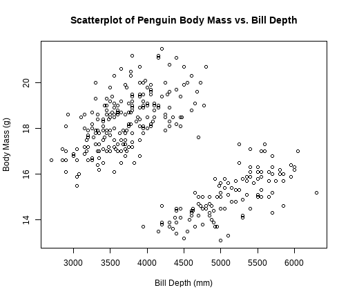
![](lab05-slides-sync_files/figure-html/massDepthPlot-1.png)
]

---
# Scatterplots: Color-Coding Points (line 97)

.pull-left[

```r
plot(bill_depth_mm ~ body_mass_g, 
     data = penguins,
     main = "Scatterplot of Penguin Body Mass vs. Bill Depth",
     xlab = "Bill Depth (mm)",
     ylab = "Body Mass (g)",
*    col = c("midnightblue", "brown1", "mediumseagreen")[penguins$species])
```

- Set `col` argument to a vector of colors
- Use `[]` to select color based on categorical variable
- Use color **with restraint**
]
.pull-right[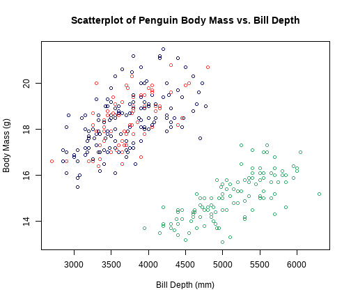
![](lab05-slides-sync_files/figure-html/speciesColor-1.png)
]

---
# Color Should Have Meaning

.pull-left[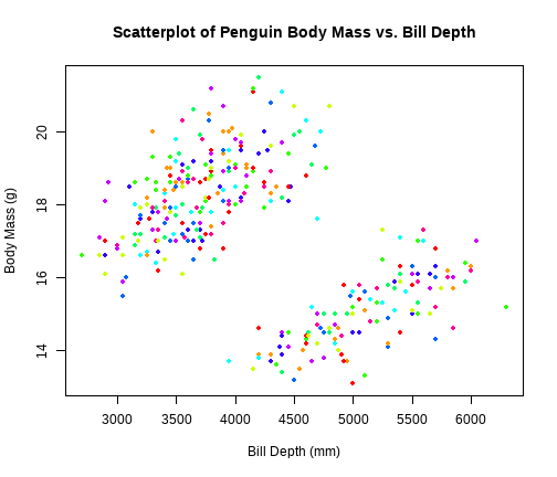
![](lab05-slides-sync_files/figure-html/tooMuchColor-1.png)
]

.pull-right[
This looks fun, but what does the color *mean*?

Color should convey information, and enhance readability.

![](https://media1.tenor.com/images/3807b6b2014638b35e047839fce2959b/tenor.gif?itemid=4897922)
]

---
# Adding Legends to Plots (line 118)

.pull-left[

```r
# Make the plot again
plot(bill_depth_mm ~ body_mass_g, 
     data = penguins,
     main = "Scatterplot of Penguin Body Mass vs. Bill Depth",
     xlab = "Bill Depth (mm)",
     ylab = "Body Mass (g)",
     col = c("midnightblue", "brown1", "mediumseagreen")[penguins$species])

# Add a legend
legend("topright", 
       legend = levels(penguins$species),
       col = c("midnightblue", "brown1", "mediumseagreen"),
*      pch = 1,
       title = "Species")
```
]
.pull-right[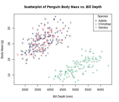
![](lab05-slides-sync_files/figure-html/legend-1.png)
]

---
# Plotting Character (`pch`, line 143)
.pull-left[

# Add a legend
legend("topright", 
       legend = levels(penguins$species),
       col = c("midnightblue", "brown1", "mediumseagreen"),
*      pch = c(0, 1, 2),
       title = "Species")
```
]
.pull-right[
![](lab05-slides-sync_files/figure-html/pchExample-1.png)
]
---
class: center,middle
# Question Break
![](https://media.tenor.com/images/7669fb21a3443e63ae29ba270b70e2a9/tenor.gif)

---
# Correlation (line 165)
.pull-left[
Last week's scatterplot:

```r
plot(body_mass_g ~ bill_length_mm,
     data = penguins,
     main = "Scatterplot of Penguin Body Mass versus Bill Length",
     xlab = "Bill Length (mm)",
     ylab = "Body Mass in (g)")
```

```r
cor(penguins$bill_length_mm, penguins$body_mass_g)
```

```
[1] 0.5894511
```
]

.pull-right[
![](lab05-slides-sync_files/figure-html/lengthMassPlot-1.png)
]

---
# Correlation Matrices (line 183)

First, subset the data to just look at quantitative variables, then feed that subset to `cor()` to compute a *correlation matrix*

```r
numericPenguins <- subset(penguins, select = c("bill_length_mm", "bill_depth_mm", "flipper_length_mm", "body_mass_g"))
cor(numericPenguins)
```

```
                  bill_length_mm bill_depth_mm flipper_length_mm body_mass_g
bill_length_mm         1.0000000    -0.2286256         0.6530956   0.5894511
bill_depth_mm         -0.2286256     1.0000000        -0.5777917  -0.4720157
flipper_length_mm      0.6530956    -0.5777917         1.0000000   0.8729789
body_mass_g            0.5894511    -0.4720157         0.8729789   1.0000000
```

Each "entry" in the correlation matrix is the correlation between the variables labeling that entry's row and column.

---
# Linear Regression (line 197)

```r
reg1 <- lm(body_mass_g ~ bill_length_mm, data = penguins)
summary(reg1)
```

```

Call:
lm(formula = body_mass_g ~ bill_length_mm, data = penguins)

Residuals:
     Min       1Q   Median       3Q      Max 
-1759.38  -468.82    27.79   464.20  1641.00

Coefficients:
               Estimate Std. Error t value Pr(>|t|)    
(Intercept)     388.845    289.817   1.342    0.181    
bill_length_mm   86.792      6.538  13.276   <2e-16 ***
---
Signif. codes:  0 '***' 0.001 '**' 0.01 '*' 0.05 '.' 0.1 ' ' 1

Residual standard error: 651.4 on 331 degrees of freedom
Multiple R-squared:  0.3475,	Adjusted R-squared:  0.3455 
F-statistic: 176.2 on 1 and 331 DF,  p-value: < 2.2e-16
```

---
# ANOVA Tables (line 214)
Give your regression model (ours is `reg1`) to the `anova()` function:

```r
anova(reg1)
```

```
Analysis of Variance Table

Response: body_mass_g
                Df    Sum Sq  Mean Sq F value    Pr(>F)    
bill_length_mm   1  74792533 74792533  176.24 < 2.2e-16 ***
Residuals      331 140467133   424372                      
---
Signif. codes:  0 '***' 0.001 '**' 0.01 '*' 0.05 '.' 0.1 ' ' 1
```

`$$R^2 = \frac{\text{SSM}}{\text{SST}}$$`
---
class:inverse
# Lab Project ⌨️

You will be **randomly** moved to a breakout room for the rest of the lab (minus ~10 minutes)

.pull-left[
### Your tasks
1. Introduce yourself to your collaborators!
1. **Work together** to complete the "Try It!" and "Dive Deeper" portions of the lab assignment by copy/pasting and modifying appropriate code from earlier in the document.
]

.pull-right[
### How to get help
- I'll be floating around between breakout rooms to check on everyone
- Use the "Ask for help" button to flag me down
- Let me know when you're done
]

---
class: center, middle, inverse
# What questions do you have? Any issues?
---
class: center, middle
# "Exit Ticket"
Please take 1-2 minutes to complete the survey at

### [bit.ly/250ticket5](http://bit.ly/250ticket5)

---
# Reminders 💡

Your tasks for the week running Friday 9/25 - Friday 10/2:

| Task | Due Date | Submission |
|:-----|:---------|:-----------|
| Homework 4 | Friday 10/2 8AM ET | course.work |
| Lab 5 | Friday 10/2 8AM ET | Canvas |

*Stop by office hours! You can attend anyone's -- not just mine!*