STATS 250 Lab 08

# STATS 250 Lab 08
## Sampling Distributions of Proportions
### Nick Seewald<br />nseewald@umich.edu
### Week of 10/19/2020

---

# Reminders 💡

Your tasks for the week running Friday 10/19 - Friday 10/23:

| Task | Due Date | Submission |
|:-----|:---------|:-----------|
| Lab 8 | Friday 10/23 8:00AM ET | Canvas |
| *No homework this week* | -- | course.work |

Office hours are back to normal this week (with a few small tweaks)

Midterm regrade requests through Gradescope due **Tuesday 10/27 8a

---
class: center

# Midterm Recap

If the midterm didn't go as expected *that's OKAY*. There's plenty of semester left.

---

# What's the plan?

Today we're going to learn about "sampling distributions" and something called the **Central Limit Theorem** (CLT).

The central limit theorem is sort of magical. We'll talk about it in more detail in lecture!

---
# Sampling Distributions

A **sampling distribution** refers to the possible values for a *statistic* (e.g., 
`$$\hat{p}$$`
) and how often those values occur.

We've sort of seen sampling distributions already. Can you think of how?

The histograms we've made of 
`$$\hat{p}_{\mathrm{sim}}$$`
are sampling distributions of 
`$\hat{p}$`
(under the null hypothesis model)!

---
class: inverse

# Penguins!

```r
penguins <- read.csv("https://raw.githubusercontent.com/STATS250SBI/palmerpenguins/master/inst/extdata/penguins_NArm.csv",
                     stringsAsFactors = TRUE)
```

---
class: inverse
# Penguins!

Let's remind ourselves of what variables are in this data:

```r
# Use your favorite function or two to explore the data
```

```r
# Use your favorite function or two to explore the data
names(penguins)
```

```
[1] "species"           "island"            "bill_length_mm"   
[4] "bill_depth_mm"     "flipper_length_mm" "body_mass_g"      
[7] "sex"               "year"             
```

> IMPORTANT NOTE: For the purposes of this example, we're going to assume that the penguins in the data represent the *population* of all penguins in the Palmer Archipelago. This is obviously not true: there are more than 333 penguins living on these islands. *This is just to illustrate ideas*.

---
# "Population" proportions

Assuming our data is on the full population of penguins in the archipelago, how could we find the population proportion of Gentoo penguins?

```r
proportions(table(penguins$species))
```

```

Adelie Chinstrap    Gentoo 
0.4384384 0.2042042 0.3573574 
```

`$$p = 0.357$$`
where `$p$` is the population proportion of Gentoo penguins in the Palmer Archipelago

---

# `set.seed()`

Start by setting the seed:

```r
set.seed(7923)
```

Things to remember when setting the seed:

- Guaranteed to get the same results from the same code in the *knitted* document
- Determines the *sequence* of random numbers: things can get knocked off sequence
- Use "Run All Chunks Above" to get back on sequence and to get the same numbers as in the knitted document

---
# Taking a sample
Take a sample of size 20 from the "population" of all penguins:

```r
sample1 <- penguins[sample(1:333, size = 20), ]
```

```
      species island bill_length_mm bill_depth_mm flipper_length_mm body_mass_g
271 Chinstrap  Dream           45.2          17.8               198        3950
252    Gentoo Biscoe           43.3          14.0               208        4575
       sex year
271 female 2007
252 female 2009
```

```r
proportions(table(sample1$species))
```

```

Adelie Chinstrap    Gentoo 
     0.50      0.15      0.35 
```

---
# Taking *another* sample

```r
sample2 <- penguins[sample(1:333, size = 20), ] # reusing the same code as above
proportions(table(sample2$species))
```

```

Adelie Chinstrap    Gentoo 
     0.65      0.20      0.15 
```

We get different results! This is expected, it's *sample-to-sample variability*.

---
# 1000 more samples
.pull-left[

```r
samplesOfSize20 <- replicate(1000, {
  s <- penguins[sample(1:333, size = 20), ]
  proportions(table(s$species))["Gentoo"]
})
```

```r
hist(samplesOfSize20,
     main = "Sampling distribution of p-hat, n = 20",
     xlab = "p-hat values",
     col = "darkturquoise",
     xlim = c(0, 1),
     cex.lab = 1.5,
     cex.main = 1.5,
     cex.axis = 1.5)
abline(v = proportions(table(penguins$species))["Gentoo"],
       lwd = 5, lty = "dashed", col = "darkblue")
```
]
.pull-right[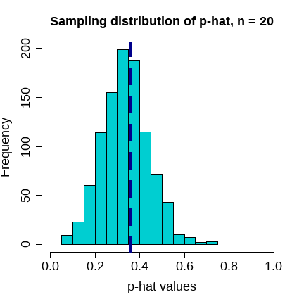
![](lab08-slides-sync_files/figure-html/samples20hist-1.png)
]

---
class: center, middle, inverse
# Describe this distribution

### https://pollev.com/nickseewald611

![](lab08-slides-sync_files/figure-html/samples20hist-1.png)

---
# Larger samples: `$n = 40$`

```r
samplesOfSize40 <- replicate(1000, {
  s <- penguins[sample(1:333, size = 40), ]
  proportions(table(s$species))["Gentoo"]
})
```

```r
hist(samplesOfSize40,
     main = "Sampling distribution of p-hat, n = 40",
     xlab = "p-hat values",
     col = "darkturquoise",
     xlim = c(0, 1),
     cex.lab = 1.5,
     cex.main = 1.5,
     cex.axis = 1.5)
abline(v = proportions(table(penguins$species))["Gentoo"],
       lwd = 5, lty = "dashed", col = "darkblue")
```
]
.pull-right[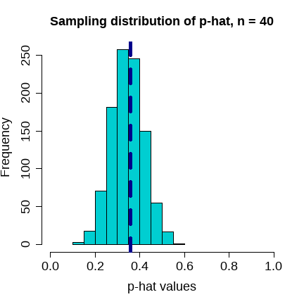
![](lab08-slides-sync_files/figure-html/samples40hist-1.png)
]

---
class: center, middle, inverse
# How do these distributions compare?

https://pollev.com/nickseewald611

.pull-left[
![](lab08-slides-sync_files/figure-html/samples20hist-1.png)
]
.pull-right[
![](lab08-slides-sync_files/figure-html/samples40hist-1.png)
]

---
# Even larger samples: `$n = 100$`

```r
samplesOfSize100 <- replicate(1000, {
  s <- penguins[sample(1:333, size = 100), ]
  proportions(table(s$species))["Gentoo"]
})
```

```r
hist(samplesOfSize100,
     main = "Sampling distribution of p-hat, n = 100",
     xlab = "p-hat values",
     col = "darkturquoise",
     xlim = c(0, 1),
     cex.lab = 1.5,
     cex.main = 1.5,
     cex.axis = 1.5)
abline(v = proportions(table(penguins$species))["Gentoo"],
       lwd = 5, lty = "dashed", col = "darkblue")
```
]
.pull-right[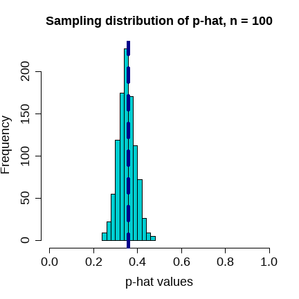
![](lab08-slides-sync_files/figure-html/samples100hist-1.png)
]

---
class:center

# Comparing Results
https://pollev.com/nickseewald611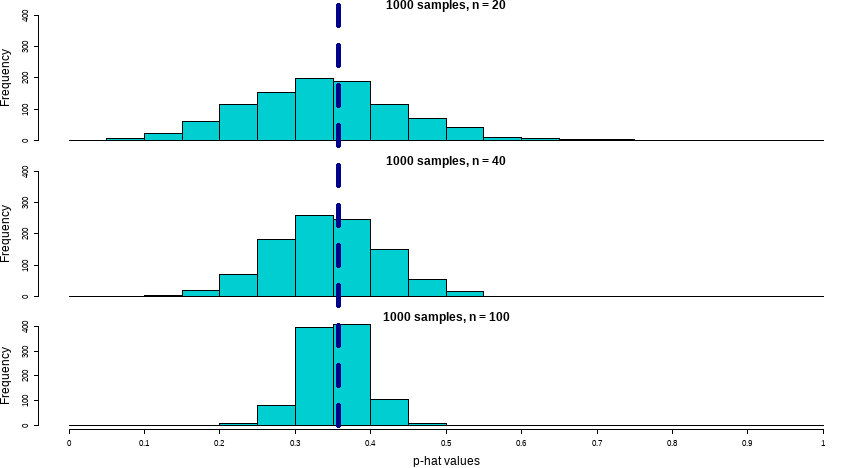
![](lab08-slides-sync_files/figure-html/histogramStack-1.png)

---
# More Detail

.pull-left[
<div style="text-align:center;"><img src="histgif/clt-proportions.gif" /></div>
]
.pull-right[
As the size of our samples increases, the sampling distribution of `$\hat{p}$` becomes...

1. more obviously centered around `$p$`
1. narrower
1. more bell-shaped
]

---
# Central Limit Theorem

> If we look at a proportion (or difference in proportions) and the scenario satisfies certain conditions, then the sample proportion (or difference in proportions) will appear to follow a bell-shaped curve called the *normal distribution*.

##Conditions:

1. **Observations in the sample are independent.** Guaranteed by random sampling or random allocation to treatment/control.
1. **The sample is large enough.** "Large enough" means `$n\times p \geq 10$` *and* `$n\times (1-p) \geq 10$` ($p$ the *population* proportion).

---
class: inverse
# Lab Project ⌨️

.pull-left[
### Your tasks
- Complete the "Try It!" and "Dive Deeper" portions of the lab assignment by copy/pasting and modifying appropriate code from earlier in the document.
- Introduce yourself to your collaborators
- **Do not leave people behind.**
]

.pull-right[
### How to get help
- Ask your collaborators -- share your screen!
- Use the "Ask for Help" button to flag me down.
]

---

# Reminders 💡

### http://bit.ly/250ticket8

Your tasks for the week running Friday 10/19 - Friday 10/23:

| Task | Due Date | Submission |
|:-----|:---------|:-----------|
| Lab 8 | Friday 10/23 8:00AM ET | Canvas |
| *No homework this week* | -- | course.work |

Office hours are back to normal this week (with a few small tweaks)

Midterm regrade requests through Gradescope due **Tuesday 10/27 8a