STATS 250 Lab 11

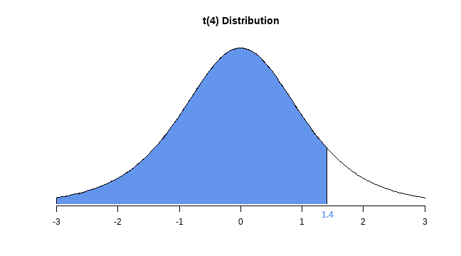
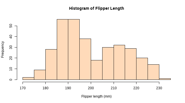
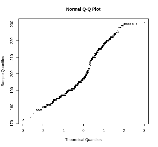
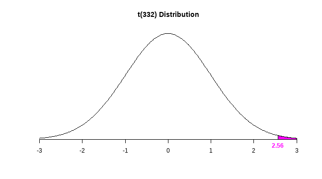
class: center, middle, inverse, title-slide

# STATS 250 Lab 11
## Confidence Intervals and Hypothesis Tests for One Mean
### Nick Seewald<br />nseewald@umich.edu
### Week of 11/9/2020

---

class: center middle

# Reminders 💡

Your tasks for the week running Friday 11/6 - Friday 11/13

| Task | Due Date | Submission |
|:-----|:---------|:-----------|
| **Quiz 2** | Monday 11/9, any 60 minutes | Canvas |
| Lab 10 | Friday 11/13 8:00AM ET | Canvas |
| Lab 11 | Friday 11/13 8:00AM ET | Canvas |
| Homework 8 | Friday 11/13 8:00AM ET | course.work |
| M-Write 2 Peer Review | Friday 11/13 4:59PM ET| Canvas

*M-Write Office Hours on Canvas!*

*No office hours today.*
---

# Homework 7 Comments

## Question 6:

.bg-washed-yellow.b--yellow.navy.ba.bw2.ph4[
According to a report on sleep deprivation by the Centers for Disease Control and Prevention, the proportion of California residents who reported insufficient rest or sleep during each of the preceding 30 days is 8.0%, while this proportion is 8.8% for Oregon residents. These data are based on simple random samples of 11,545 California and 4,691 Oregon residents.

- Check the appropriate conditions for this confidence inteval.
- Calculate a 95% confidence interval for the difference between the proportions of Californians and Oregonians who are sleep deprived.
- Interpret your interval in context of the data.
]

---
# Homework 7 Comments

## Question 6:
- Remember that conditions are
  - `$n_1 \times p_1 \geq 10$`, `$n_1 \times (1 - p_1) \geq 10$`
  - `$n_2 \times p_2 \geq 10$`, `$n_2 \times (1-p_2) \geq 10$`
  - independent random samples

- Make sure to compute a 95% CI using `$z^* = 1.96$`

- Interpretation of a confidence interval must state confidence *level*

---
# Homework 7 Comments

## Question 7a:

.bg-washed-yellow.b--yellow.navy.ba.bw2.ph4[
Researchers studying the link between prenatal vitamin use and autism surveyed the mothers of a random sample of children aged 24 - 60 months with autism and conducted another separate random sample for children with typical development. The table below shows the number of mothers in each group who did and did not use prenatal vitamins during the three months before pregnancy (periconceptional period).

State appropriate hypotheses to test for independence of use of prenatal vitamins during the three months before pregnancy and autism.
]

---
# Homework 7 Comments

## Question 7a:

- Questions about "rates" should be about proportions

- `$H_0: \ p_{\text{vitamin}} = p_{\text{no vitamin}}$` vs. `$H_a: \ p_{\text{vitamin}} \neq p_{\text{no vitamin}}$`, where `$p_x$` is the population proportion of children with autism in group `$x$`.
  - When we say "test for independence" that doesn't specify a direction for the alternative.
  - `$H_0: \ p_{\text{autism}} = p_{\text{no autism}}$` vs. `$H_a: \ p_{\text{autism}} \neq p_{\text{no autism}}$` is also okay, provided you then re-define `$p_x$`
  
---
# Homework 7 Comments

## Question 7b:

.bg-washed-yellow.b--yellow.navy.ba.bw2.ph4[
Complete the hypothesis test and state an appropriate conclusion. (Reminder: verify any necessary conditions for the test.)
]

- **Check conditions:** independent random samples, `$\geq 10$` successes/failures in each group
- This is a *two-sided test*: double the one-sided `$p$`-value!
- Conclusions must be **in context**.

---
# The `$t$` distribution

- Bell-shaped
- Heavier tails than the normal distribution
- Used to approximate `$N(0, 1)$`.

---
# The `$t$` distribution

We can use `pt()` and `qt()` just like `pnorm()` and `qnorm()`:

.pull-left[

```r
pt(q = 1.4, df = 4)
```

```
[1] 0.8829497
```

```r
qt(0.8829, df = 4)
```

```
[1] 1.399641
```

```r
plotT(df = 4, 
      shadeValues = 1.4,
      direction = "less")
```
]

.pull-right[
![](lab11-slides-sync_files/figure-html/pt1-plot-1.png)
]
---
class: inverse

# Penguins! (line ~68)

```r
penguins <- read.csv("https://raw.githubusercontent.com/STATS250SBI/palmerpenguins/master/inst/extdata/penguins_NArm.csv",
                     stringsAsFactors = TRUE)
```

---
# Let's make a confidence interval

Let's say we want to construct a confidence interval for the population mean flipper length of penguins living in the Palmer Archipelago, or conduct a hypothesis test for that mean.

--
In order to use our machinery for constructing confidence intervals and performing hypothesis tests for means, we need two conditions to hold. **What are they?** (type in chat)
--

1. **Random sample:** the penguins in our sample are selected independently of one another.
2. **Nearly-normal data:** The flipper lengths need to be approximately normally-distributed

---
class:center, middle
# Nick's Fundamental Question of Statistics

.bg-washed-yellow.b--yellow.navy.ba.bw2.ph4[
The most important question in statistics is not whether you .b[can] do something, it's whether you .b[should] do it.
]

This means that checking conditions is **hugely important**.

---
# Checking Conditions

1. **Independent Observations:** There are 333 penguins in the data set; there are probably more than 3,330 penguins in the Palmer archipelago. We don't know exactly the sampling mechanism, though, so we'll proceed with caution.
--

2. **Nearly-Normal Data:** One way to do this is to look at a histogram.

.pull-left[

```r
hist(penguins$flipper_length_mm,
     main = "Histogram of Flipper Length",
     xlab = "Flipper length (mm)",
     col = "peachpuff")
```

**What are your thoughts about this histogram?**
]
.pull-right[
![](lab11-slides-sync_files/figure-html/flipperHist-1.png)
]

---
# Q-Q Plots (line ~99)

.pull-left[
Another way to check the nearly-normal condition

- Actual data on **y-axis** ("sample quantiles")
- What that data would look like if it came from a normal distribution on **x-axis** ("theoretical quantiles").
- Straight line with positive slope `$\Rightarrow$` 
data come from a normally-distributed population

```r
qqnorm(penguins$flipper_length_mm)
```
]

.pull-right[
![](lab11-slides-sync_files/figure-html/flipperQQ-1.png)
]

---
# Q-Q Plots (line ~110)

```r
qqnorm(penguins$flipper_length_mm)
qqline(penguins$flipper_length_mm, col = "blue", lwd = 2)
```

**What should we conclude from this Q-Q plot?**

---
# Can we proceed?

- The data are pretty clearly bimodal.
- **BUT** we've got a lot of data (n = 333).

.bg-washed-yellow.b--yellow.navy.ba.bw2.ph4[
.b[Central limit theorem:] When we have a "large enough" sample size, the sampling distribution of `$\bar{x}$` (the sample mean) will be *nearly normal*: `$\bar{x}$` will have a `$N(\mu, \sigma/\sqrt{n})$` distribution.
]

- Is `$n=333$` large enough?
--

YES.

---
# `t.test()`

Let's construct a 90% confidence interval for the population mean flipper length of penguins living in the Palmer Archipelago.

--
.pull-left[
Let's look at some summary statistics:

```r
summary(penguins$flipper_length_mm)
```

```
   Min. 1st Qu.  Median    Mean 3rd Qu.    Max. 
    172     190     197     201     213     231 
```
]
--

.pull-right[

```r
t.test(penguins$flipper_length_mm,
       conf.level = 0.9)
```

```

One Sample t-test

data:  penguins$flipper_length_mm
t = 261.66, df = 332, p-value < 2.2e-16
alternative hypothesis: true mean is not equal to 0
90 percent confidence interval:
 199.7001 202.2338
sample estimates:
mean of x 
  200.967 
```
]

---
# `t.test()`
.pull-left[
- Holy `$p$`-value, Batman!
- `2.2e-16` is as small a number as R can make

- Hypotheses are set up to be about `$\mu = 0$`: does this make sense?
- `$t = \frac{\bar{x} - \mu}{s/\sqrt{n}}$`
]
.pull-right[

```r
t.test(penguins$flipper_length_mm,
       conf.level = 0.9)
```

```

One Sample t-test

---
# `t.test()`

Let's test `$H_0: \mu = 199$` vs. `$H_a: \mu > 199$`. To do this, we'll provide the `mu` and `alternative` arguments to `t.test()`:

.pull-left[

```r
t.test(penguins$flipper_length_mm,
*      mu = 199,
*      alternative = "greater")
```

```

One Sample t-test

data:  penguins$flipper_length_mm
t = 2.561, df = 332, p-value = 0.00544
alternative hypothesis: true mean is greater than 199
95 percent confidence interval:
 199.7001      Inf
sample estimates:
mean of x 
  200.967 
```
]
.pull-right[

```r
plotT(df = 332, shadeValues = 2.561,
      direction = "greater", col.shade = "magenta")
```
![](lab11-slides-sync_files/figure-html/t.test2Plot-show-1.png)
]

---
# Two Important Notes

.bg-washed-yellow.b--yellow.navy.ba.bw2.ph4[
Everything you've learned about proportions in terms of interpretation of CI's and hypothesis tests .b[stays the same]. The only thing that changes is the fact that .b[the parameter is now a a population mean].
]

.navy[]

.bg-washed-yellow.b--yellow.navy.ba.bw2.ph4[
Bimodal distributions are generally pretty clear indicators of the presence of an important subgroup. Flipper length is probably related to species; we should investigate that relationship further!
]
---
class: inverse
# Code Cheat Sheet 💻
### **`pt(q, df, lower.tail = TRUE)`**
  - `q` is the x-axis value you want to find an area related to
  - `df` is the degrees of freedom of the `$t$` distribution
  - `lower.tail` determines whether `pt()` finds the area to the left or right of `q`. If `lower.tail = TRUE` (the default), it shades to the left. If `lower.tail = FALSE`, it shades to the right.

---
class: inverse
# Code Cheat Sheet 💻
### **`qt(q, df, lower.tail = TRUE)`**
  - `p` is the probability or area under the curve you want to find an x-axis value for
  - `df` is the degrees of freedom of the `$t$` distribution
  - `lower.tail` determines whether `pt()` finds the area to the left or right of `q`. If `lower.tail = TRUE` (the default), it shades to the left. If `lower.tail = FALSE`, it shades to the right.
  
---
class: inverse
# Code Cheat Sheet 💻
### **`plotT()`**
  - `df` refers to the degrees of freedom of the distribution to plot. You must provide this value.
  - `shadeValues` is a vector of up to 2 numbers that define the region you want to shade
  - `direction` can be one of `less`, `greater`, `outside`, or `inside`, and controls the direction of shading between `shadeValues`. Must be `less` or `greater` if `shadeValues` has only one element; `outside` or `inside` if two
  - `col.shade` controls the color of the shaded region, defaults to `"cornflowerblue"`
  - `...` lets you specify other graphical parameters to control the appearance of the normal curve (e.g., `lwd`, `lty`, `col`, etc.)

---
class: inverse
# Code Cheat Sheet 💻
###  **`qqnorm(y, ...)`**
  - `y` refers to the variable for which you want to create a Q-Q plot
  - `...` lets you control graphical elements of the plot like `pch`, `col`, etc.

### **`qqline(y, ...)`**
  - `y` refers to the variable for which you created a Q-Q plot
  - `...` lets you control graphical elements of the plot like `pch`, `col`, etc.
  - Function can only be used *after* using `qqnorm()`
  
---
class: inverse
# Code Cheat Sheet 💻
###  **`t.test(x, alternative = c("two.sided", "less", "greater"), mu = 0, conf.level = 0.95)`**
  - `x` is a vector of data values
  - `alternative` specifies the direction of the alternative hypothesis; must be one of "two.sided", "less", or "greater"
  - `mu` indicates the true value of the mean (under the null hypothesis); defaults to 0
  - `conf.level` is the confidence level to be used in constructing a confidence interval; must be between 0 and 1, defaults to 0.95

---
class: inverse
# Lab Project ⌨️

.pull-left[
### Your tasks
- Complete the "Try It!" and "Dive Deeper" portions of the lab assignment by copy/pasting and modifying appropriate code from earlier in the document.
- Introduce yourself to your collaborators
- **Do not leave people behind.**
]

.pull-right[
### How to get help
- Ask your collaborators -- share your screen!
- Use the "Ask for Help" button to flag me down.
]

---
class: center, middle

# How'd it go? Questions?

### http://bit.ly/250ticket11

---
class: center middle

# Reminders 💡

Your tasks for the week running Friday 11/6 - Friday 11/13

*M-Write Office Hours on Canvas! No office hours today.*